I have been collecting anonymous pharmacokinetic data from rxkinetics.net for the past 13 years. I last analyzed this dataset in March 2016 and published the results in a blog post titled “Data Mining.” On the tenth anniversary of that post, I revisited the data.

Note the dataset is intentionally minimal, including only date, model used, age, gender, height, weight, serum creatinine, creatinine clearance (CrCL), elimination rate (Kel), and volume of distribution (Vd). Also, there is no formal quality control applied to these data. As a result, some entries may be fictional, incorrectly entered, or duplicated. The data were collected anonymously, in accordance with our website privacy policy, from registered users worldwide.

Descriptive stats

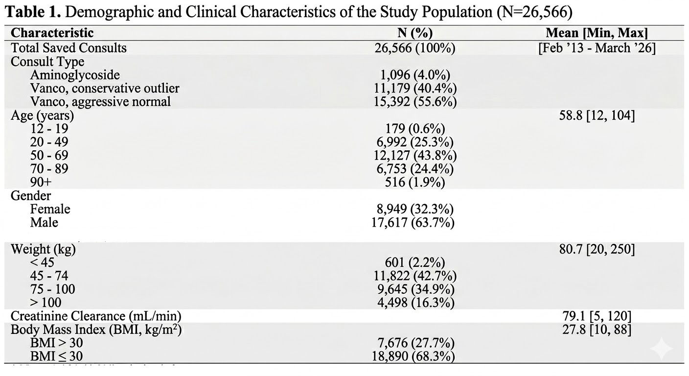
Several inferences can be drawn from the descriptive statistics.

In September 2019, I changed the vancomycin model labels from “normal/outlier” to “aggressive/conservative.” Prior to this change, the selection ratio of normal to outlier models was 6.67:1. After the change, the ratio of aggressive to conservative shifted to 0.84:1. As suspected, the original model names were likely misleading for users who were unfamiliar with the distinctions and appropriate use of each model.

The BMI distribution (<30% excess BMI) suggests that a substantial portion of the data may originate from outside the United States.

Males outnumber females approximately 2:1. This likely reflects a data entry bias, as “male” is the default selection, suggesting that users may not be consistently updating the field when entering female patients.

Data analysis

Because most of the data pertained to vancomycin, I filtered the dataset to include only those records. Also, I excluded a small number of clearly implausible data points. This included six cases with BMI > 100 accompanied by unrealistically low height values, likely reflecting data entry error (though clinical scenarios such as amputations cannot be ruled out). There were 624 records with a half-life < 4 hours and 15 with a half-life > 7 days, some of which were associated with relatively normal creatinine clearance. The underlying reason for such results cannot be determined, as the serum concentration values and sampling times used for these calculations were not retained. After removing these extreme values, the final dataset consisted of 25,585 observations.

All record analysis

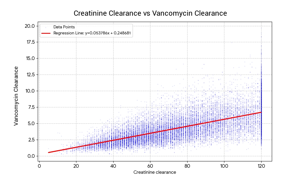
Regression analysis results: the relationship between Creatinine clearance (CrCL) and vancomycin clearance (VanCL) is defined by the following linear equation:

VanCL = (0.053786 x CrCL) + 0.248681

Correlation (r): 0.6711
• Indicates a solid positive linear relationship between the two variables.
Coefficient of Determination (R^2): 0.4504
• This means about 45% of the variation in VanCL is explained by the change in CrCL
Significance (P-value): < 0.0001
• The relationship is highly statistically significant.
Standard Error (RMSE): 1.7308

The residual plot shows the difference between the actual observed values and the values predicted by our model. Interpretation: A random scatter around the red zero line suggests that the linear model is appropriate for this data.

The histogram of residuals shows how the “errors” (residuals) are distributed. The bell-shaped curve indicates that the errors are normally distributed, which validates the use of linear regression for this dataset.

Comparative Analysis

Next, I broke the data into two groups. Group 1: BMI 30 or less (n=18,329) and Group 2: BMI greater than 30 (n=7,456).

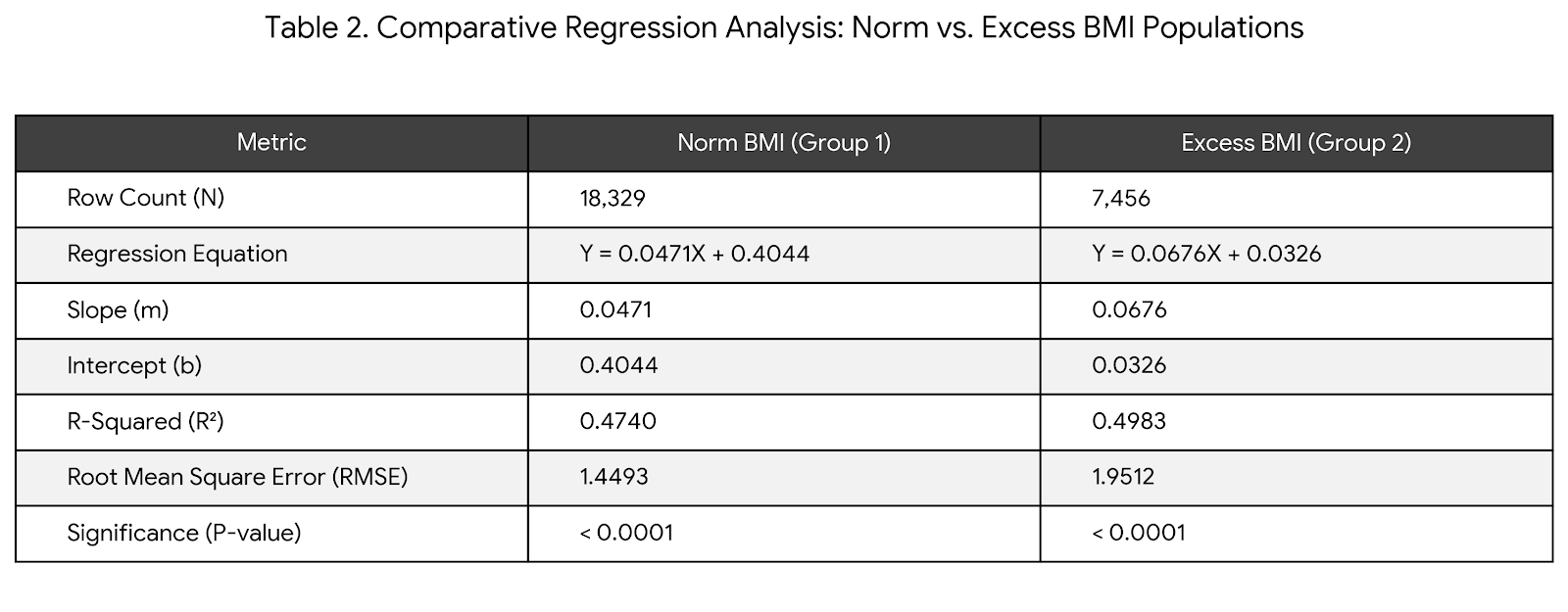
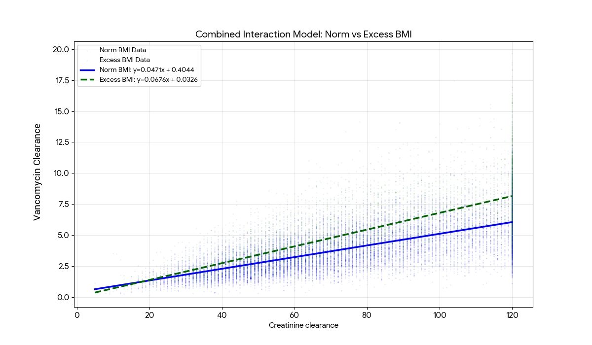
Regression results:
• Group 1: Y = 0.047057X + 0.404398
• Group 2: Y = 0.067640X + 0.032623

Key Differences and Findings

1. Change in Slope:
   The slope increased significantly from Group 1 to Group 2 (0.047 -> 0.068).
   This suggests that in the second group, for every unit increase in Creatinine clearance, the increase in VanCL is nearly 44% higher than in the first group.
2. Intercept Shift:
   The intercept dropped significantly (0.40 -> 0.03).
   This implies that at very low renal function (Creatinine clearance near 0), the starting value for VanCL is much lower in Group 2.
3. Model Strength (R^2):
   Group 2 fits the linear model slightly better than Group 1 (49.8% vs 47.4%).
4. Error Margin (RMSE):
   Group 2 has a higher RMSE (1.95 vs 1.45), meaning the data points are more widely dispersed around the regression line than Group 1.

Chow Test Results
Results testing the null hypothesis (H0): The coefficients (slope and intercept) are identical for both groups:

• F-Statistic: 1996.62
• P-Value: < 0.0000000001 (1.11 x 10^-16)

Since the p-value is essentially zero, the null hypothesis is rejected. This confirms a “structural break” in the data. The way CrCL predicts VanCL in Group 1 is mathematically different from how it predicts VanCL in Group 2.

Because the Chow Test is significant, we cannot use a single linear equation to describe both groups accurately. Predictions would be consistently biased (over-predicting for one group and under-predicting for the other).

The Chow Test confirms that the two groups of data are statistically distinct. The relationship between CrCL and VanCL is not the same for both datasets.

Comparative Population Model Performance

Let’s look at how each of the two population models, C and K, perform with each group: (1) BMI 30 or less (n=18,329) and (2) BMI greater than 30 (n=7,456).. Model C is labeled “conservative” in the app and calculates vancomycin clearance. Model K is labeled “aggressive” in the app and calculates vancomycin Kel and Vd separately.

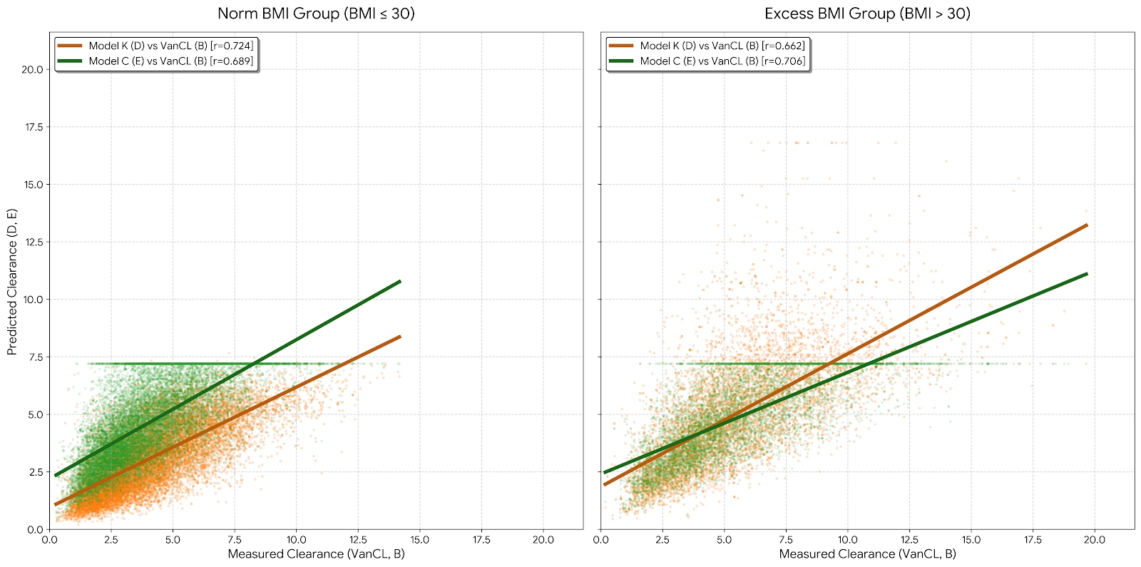
Group	Model K (r)	Model C (r)	Performance
Norm BMI (<= 30)	0.724	0.689	Model K is the stronger predictor.
Excess BMI (> 30)	0.662	0.706	Model C is the stronger predictor.

Our analysis shows that a one-size-fits-all modeling approach is flawed. For patients with a BMI <= 30, Model K (labeled “aggressive” in the app) is the statistically superior predictor of drug clearance. However, once a patient crosses the BMI threshold of 30, Model C (labeled “conservative” in the app) takes the lead.

Clinicians should be aware that model reliability is not static; it fluctuates based on the patient’s body mass, with all models becoming less reliable as obesity increases. This means that as BMI increases, the ‘safety net’ provided by mathematical formulas becomes significantly thinner, demanding more frequent serum monitoring.